Simple nonlinear prediction

  Conventional linear prediction schemes average over all locations in phase space when they extract the correlations they exploit for predictability. Tong [42] promoted an extension that fits different linear models if the current state is below or above a given threshold (TAR, Threshold Autoregressive Model). If we expect more than a slight nonlinear component to be present, it is preferable to make the approximation as local in phase space as possible. There have been many similar suggestions in the literature how to exploit local structure, see e.g. [43, 44, 45, 46]. The simplest approach is to make the approximation local but only keep the zeroth order, that is, approximate the dynamics locally by a constant. In the TISEAN package we include such a robust and simple method: In a delay embedding space, all neighbors of are saught, if we want to predict the measurements at time n+k. The forecast is then simply
 
i.e. the average over the ``futures'' of the neighbors. The average forecast errors obtained with the routine zeroth (predict would give similar results) for the laser output data used in Fig.  as a function of the number k of steps ahead the predictions are made is shown in Fig. . One can also iterate the predictions by using the time series as a data base.

 
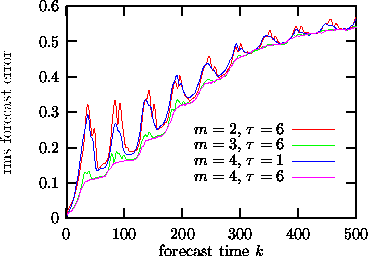
Figure:   Predictions k time steps ahead (no iterated predictions) using the program zeroth. Top (red) curve: embedding dimension two is insufficient, since these flow data fill a (2+)-dimensional attractor. Second from top (blue): Although embedding dimension four should in theory be a good embedding, suppresses structure perpendicular to the diagonal so that the predictions are as bad as in m=2! Lower (green, pink) curves: m=3 and 4 with a delay of about 4-8 time units serve well.

Apart from the embedding parameters, all that has to be specified for zeroth order predictions is the size of the neighborhoods. Since the diffusive motion below the noise level cannot be predicted anyway, it makes sense to select neighborhoods which are at least as large as the noise level, maybe two or three times larger. For fairly clean time series, this guideline may result in neighborhoods with very few points. Therefore zeroth also permits to specify the minimal number of neighbors to base the predictions on.

A relevant modification of this method is to extend the neighborhood to infinity, but to introduce a distance dependent weight,
 
where w is called the kernel. For where is the Heaviside step function, we return to Eq.().